Example usage

The following example requires that the MDAnalysisTests datafiles and seaborn packages are installed. Both of these can be installed through pip:

pip install MDAnalysisTests seaborn

pKa estimates from a molecular dynamics trajectory

We first import the paths to the test topology and trajectory and load them into an MDAnalysis Universe. This universe contains a trajectory of an adenylate kinase protein with 3341 atoms and 214 residues.

import MDAnalysis as mda
from MDAnalysisTests.datafiles import PSF, DCD

u = mda.Universe(PSF, DCD)

The pKa estimates of are generated by the PropkaTraj analysis class

import propkatraj

pkatraj = propkatraj.PropkaTraj(u)
pkatraj.run()

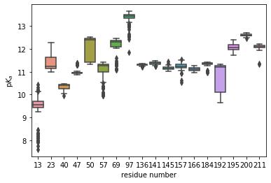
Once the run method has finished executing, the resulting pKa estimates, a function of residue number and time, can be found in the pkatraj.results.pkas as a panda dataframe. The columns of the dataframe are the residue numbers and the DataFrame index is the time in nanoseconds. These data can be visualized using matplotlib and seaborn:

import matplotlib.pyplot as plt
import seaborn as sns

fig = plt.figure(figsize=(28, 8))
ax = fig.add_subplot(1,1,1)
sns.boxplot(data=pkatraj.results.pkas, ax=ax)
ax.set_xlabel("residue number")
ax.set_ylabel(r"p$K_a$")
plt.show()

Residues can easily be selected by using information stored in the original Universe. For instance, assume we are only interested in the pKa distribution of the protein’s lysines. We can select all lysine residues by name and collect their resids, which are the columns in the DataFrame.

resides = u.select_atoms('resname LYS').residues.resids

sns.boxplot(data=pkatraj.results.pkas[resids])
ax = plt.gca()
ax.set_xlabel('residue number')
ax.set_ylabel(r'p$K_a$')
plt.show()